R에서 해보는 한국 일제강점기 시의 단어 분석
- 본 포스트는 Single World Analysis of Early 19th Century Poetry Using tidytext의 내용을 수정, 발전시킨 것입니다. 분석 방법은 기본적으로 모두 원 블로그에서 따온 것임을 밝힙니다.
- 전희원님의 KoNLP는 정말 멋진 패키지이지만, 본문에서는 적용하지 않았습니다. 다음번 포스팅에는 독자분들이 좀 더 쉽게 접근하실 수 있도록 KoNLP를 통한 분석도 싣도록 하겠습니다.
- 여기에서는 코모란 3.0을 적용했습니다. 아쉽게도 R 포팅은 없기 때문에, rJava interface를 통해 Komoran 3.0 Java Archive를 직접 불러와 태깅했습니다.
- 본문에서 사용한 감정사전은 두 종류입니다. 하나는 NRC Emoticon Lexicon이며, 다른 하나는 Bing Opinion Lexicon입니다. 전자는 Saif Mohammad에게 이메일을 통해 사용 허가를 받았으며, 후자는 자료가 공개 형태로 올라와 있어 특별히 허가를 받지는 않았습니다.
Tidy text? 낱개 단어 분석이란?
최근 자연어 처리(NLP, Natural Language Process)에서 가장 주목받는 기술은 Word Embedding일 것 같습니다. 단어를 벡터 공간에 배치하여 딥러닝에 적합한 자료 형태로 텍스트를 변형시키는 방법으로 주목받은 Word Embedding은 뛰어난 기법임에는 틀림없지만, 아직 개별 단어 또는 글뭉치의 분석에 적용할 방법은 잘 모르겠습니다. 예컨대 글뭉치의 주제 분석에 활용하는 LDA(Latent Dirichlet Analysis)에 Word Embedding을 적용하는 LDA2Vec 등이 제시었지만 성공적이라고 보기는 어려운 것 같습니다.
한편 최근 R 진영에서 텍스트 분석은 tidytext가 점차 두각을 나타내고 있는 것 같습니다. Julia Silge와 David Robinson이 만든 패키지이자 둘의 공저인 Text Mining with R에 잘 설명되어 있는 tidytext는 텍스트 자료를 tidy data 형태로 정리하여 분석하는 방법을 제공합니다. dplyr등으로 R을 현재의 반열에 올려놓은 (개인적 의견입니다만) Hadley Wickham이 정리한 tidy data의 개념을 보면 다음과 같습니다.
- 각 변수를 열에 배치
- 각 관찰값은 행에 배치
- 관찰 단위 별로 테이블 제작
이 원칙을 텍스트 분석에 적용하면, 한 열에 하나의 토큰이 배치되어 있는 테이블을 만드는 것을 의미할 겁니다. 토큰은 텍스트의 의미 단위로, 단어 하나, 형태소 하나, 어절 하나 등 분석 방법에 따라 달라지게 될 겁니다. 보통 하나의 단어를 한 열에 두지만, n-gram의 경우에는 좀 달라질 것 같고, 텍스트를 통째로 자료로 넣는 경우에는 또 다르겠지요.
예를 볼게요. (tidytextmining.com, Chapter 1에서 가져온 예제입니다.)
text <- c("Because I could not stop for Death -",
          "He kindly stopped for me -",
          "The Carriage held but just Ourselves -",
          "and Immortality")
디킨슨의 시 일부입니다. 일단 tidy text dataset으로 만들기 위해서는, 자료를 data frame으로 바꿔야 합니다.
library(tidyverse)

text_df <- data_frame(line=1:4, text=text)

text_df
## # A tibble: 4 × 2
## line text
## <int> <chr>
## 1 1 Because I could not stop for Death -
## 2 2 He kindly stopped for me -
## 3 3 The Carriage held but just Ourselves -
## 4 4 and Immortality
tibble은 R base data frame의 수정판입니다. data.frame 함수가 아닌 data_frame 함수를 사용하고, dplyr 패키지의 여러 함수를 적용해 테이블을 변형하기 무척 쉬워집니다.
library(tidytext)

text_df %>%
  unnest_tokens(word, text)
## # A tibble: 20 × 2
## line word
## <int> <chr>
## 1 1 because
## 2 1 i
## 3 1 could
## 4 1 not
## 5 1 stop
## 6 1 for
## 7 1 death
## 8 2 he
## 9 2 kindly
## 10 2 stopped
## 11 2 for
## 12 2 me
## 13 3 the
## 14 3 carriage
## 15 3 held
## 16 3 but
## 17 3 just
## 18 3 ourselves
## 19 4 and
## 20 4 immortality
이렇게 토큰(여기에서는 단어) 별로 텍스트를 나열한 것을 tidy text format이라고 합니다. 물론 tm 패키지로 document-term matrix를 만들거나 할 때에는 자료형을 다시 변형시켜야 겠지만, 일단 여기에서는 감정 분석을 진행할 것이기 때문에 여기까지만 말씀드려도 충분할 것 같습니다. 다음 번에 LDA를 다룰 때 다시 설명드릴게요.
제가 이 분석을 진행하면서 참고한 블로그는 이렇게 tidy text format으로 정리한 낱개 단어를 바탕으로 분석을 진행하는 것에 낱개 단어 분석(single word analysis)이라는 이름을 붙였던데, 이 표현이 통용되는지는 잘 모르겠습니다. Tidy text analysis로 충분한 것 같은데 굳이 다른 이름을 붙일 이유가 있을까요.
진행 순서: 한국 근대시 감정분석
- http://biblio.endy.pe.kr/ scraping module 제작
- NRC emotion lexicon, Bing lexicon 번역
- Komoran 3.0 interface by rJava
- 분석 및 display
한국 근대시 도서관 scraping module
한국 근대시 도서관에는 저작권이 만료된 시집 김억 <시선>, 윤동주 <하늘과 바람과="" 별과="" 시="">, 한용운 <님의 침묵="">과 시 최남선 <해에게서 소년에게="">가 게제되어 있습니다. 저작권 만료로 인터넷에 공개되어 있는 시선이므로, 분석하는 데에 문제는 없습니다. 단, 총 31편으로 자료가 부족하다는 단점이 있으며, 다음번에는 [위키문헌](https://ko.wikisource.org/wiki/위키문헌:대문) scraping module을 통해 더 많은 텍스트를 분석해 보도록 하겠습니다.
library(tidyverse)
library(tidytext)
library(stringr)
library(rvest)
library(extrafont)
library(rJava)
library(translate)
사용한 패키지입니다. rJava는 Komoran 3.0을 불러오기 위해, translate는 Google Translate API를 연결해 사전을 번역하는데 사용합니다. extrafont는 그래프의 폰트 변경 때문에 불렀습니다.
base_url <- "http://biblio.endy.pe.kr"

poem_link <- str_c(base_url, "/home") %>%
  read_html() %>%
  html_nodes(xpath="//li//div//a[@class='sites-navigation-link']") %>%
  html_attr("href")
먼저 첫 페이지에서 각 시의 링크를 뽑아옵니다. poem_link에 각 시로 연결되는 링크를 받아 (html_attr("href")) 저장합니다. 해당 사이트는 아쉽게도 페이지가 완전히 규칙적이지는 않습니다. 처음부터 조금 문제에 부딪힙니다.
gim_eog_poem <- poem_link[2:14]
yundongju_poem <- poem_link[16:21]
choenamseon_poem <- poem_link[22]
hanyongun_poem <- poem_link[24:35]
시를 규칙으로 뽑아올 수가 없어서, 수작업으로 일단 분류했습니다. 중간 중간 빠진 열은 시집의 소개가 들어있는 페이지의 링크이기 때문에 제외했습니다.
get_poem <- function(poem_url) {

  base_url <- "http://biblio.endy.pe.kr"

  # 주소와 앞에서 추출한 시의 링크를 결합, 시 본문에 접근합니다.
  # 원문 텍스트를 추출합니다.
  poem_body <- str_c(base_url, poem_url) %>%
    read_html() %>%
    html_nodes(xpath="//table[@class='sites-layout-hbox']//tbody//tr//td") %>%
    "["(., length(.)) %>%
    html_children() %>%
    html_text()

  # 첫 줄이 제목이고 조금 특이한 whitespace인 \u3000으로 구분되어 있어, regular expression으로 제목을 추출한 다음 나머지를 시 본문으로 삼습니다.
  title <- regmatches(poem_body, regexpr('[ ㄱ-ㅎ가-힣]*[\u3000]', poem_body))
  poem_body <- sub('[ ㄱ-ㅎ가-힣]*[\u3000]', ' ', poem_body)

  # 제목에서 두 칸 이상의 빈 공간, 특수문자, 한자 등을 제거합니다.
  title <- str_replace_all(title, pattern="\r", replacement="") %>%
    str_replace_all(pattern="\n", replacement=" ") %>%
    str_replace_all(pattern="[\u3000]", replacement="") %>%
    str_replace_all(pattern="[  ]{2}", replacement="") %>%
    str_replace_all(pattern="[[:punct:]]", replacement=" ") %>%
    str_replace_all(pattern="[\u4E00-\u9FD5○]", replacement="") %>%
    str_trim(side="both")

  # 마찬가지로 본문에서 두 칸 이상의 빈 공간, 특수문자, 한자 등을 제거합니다.
  poem_body <- str_replace_all(poem_body, pattern="\r", replacement="") %>%
    str_replace_all(pattern="\n", replacement=" ") %>%
    str_replace_all(pattern="[\u3000]", replacement=" ") %>%
    str_replace_all(pattern="[  ]{2}", replacement="") %>%
    str_replace_all(pattern="[[:punct:]]", replacement=" ") %>%
    str_replace_all(pattern="[\u4E00-\u9FD5○]", replacement="")

  return(list(title=title, body=poem_body))
}
시를 받아오는 기본 함수입니다. Argument로 위에서 만든 시 링크를 받아, 각 시의 본문을 scraping합니다. R은 여러 값을 동시에 반환할 수 없기 때문에, 리스트 형태로 자료를 묶어 반환합니다. 통일된 양식이 아니라서 scraping이 매우 어려월습니다. 또, 김억 시인의 발문 ‘시형의 음률과 호흡’, 한용운 시인의 ‘나의 길’은 제목이 자동으로 수집되지 않습니다.
gim_eog_date <- function(poem_url) {
  base_url <- "http://biblio.endy.pe.kr"

  # 다시 본문을 받아옵니다.
  poem_body <- str_c(base_url, poem_url) %>%
    read_html() %>%
    html_nodes(xpath="//table[@class='sites-layout-hbox']//tbody//tr//td") %>%
    "["(., 1) %>%
    html_children() %>%
    html_text()

  # regular expression으로 네자리 숫자를 추출합니다.
  date <- regmatches(poem_body, regexpr('[0-9]{4}', poem_body))

  return(date)
}
김억 시인의 경우에는 본문에 쓰인 날짜가 적혀 있어, 추출하기 위한 루틴을 추가했습니다. 물론 기본 scraping 함수에 합쳐도 되지만, 좀 더 단순하게 코드를 짜고 싶었습니다.
get_yundongju_poem <- function(poem_url) {

  # 윤동주 시인의 시를 scraping하기 위한 module

  base_url <- "http://biblio.endy.pe.kr"

  poem_body <- str_c(base_url, poem_url) %>%
    read_html() %>%
    html_nodes(xpath="//table[@class='sites-layout-hbox']//tbody//tr//td") %>%
    "["(., 1) %>%
    html_children() %>%
    html_text()

  # 제목, 쓰인 날짜를 추출합니다.
  title <- regmatches(poem_body, regexpr('[ ㄱ-ㅎ가-힣\u4E00-\u9FD5]+[\n]{2}', poem_body))
  poem_date <- regmatches(poem_body, regexpr('[\u4E00-\u9FD5○]{4}', poem_body))
  poem_body <- sub('[ ㄱ-ㅎ가-힣\u4E00-\u9FD5]*[\n]{2}', ' ', poem_body)

  # 제목을 정리합니다.
  title <- str_replace_all(title, pattern="\r", replacement="") %>%
    str_replace_all(pattern="\n", replacement=" ") %>%
    str_replace_all(pattern="[\u3000]", replacement="") %>%
    str_replace_all(pattern="[  ]{2}", replacement="") %>%
    str_replace_all(pattern="[[:punct:]]", replacement=" ") %>%
    str_replace_all(pattern="[\u4E00-\u9FD5○]", replacement="") %>%
    str_trim(side="both")

  # 본문을 정리합니다.
  poem_body <- str_replace_all(poem_body, pattern="\r", replacement="") %>%
    str_replace_all(pattern="\n", replacement=" ") %>%
    str_replace_all(pattern="[\u3000]", replacement="") %>%
    str_replace_all(pattern="[  ]{2}", replacement="") %>%
    str_replace_all(pattern="[[:punct:]]", replacement=" ") %>%
    str_replace_all(pattern="[\u4E00-\u9FD5○]", replacement="")

  # 쓰인 날짜가 한문으로 되어 있어, 한글로 바꿉니다.
  # 더 쉬운 방법이 있으면 알려주시면 감사하겠습니다.
  poem_date <- str_replace_all(poem_date, "一", "1") %>%
    str_replace_all("三", "3") %>%
    str_replace_all("四", "4") %>%
    str_replace_all("九", "9") %>%
    str_replace_all("○", "0")

  return(list(title=title, body=poem_body, date=poem_date))
}
윤동주 시인의 시는 배치가 달라, 별도로 함수를 만들었습니다.
Emotion lexicon과 Komoran 3.0
서두에 말씀드린대로, NRC emotion lexicon과 Bing opinion lexicon을 사용하여 감정 분석에 들어갑니다. 제작년에는 오픈한글에서 한글 감정 어휘를 확인할 수 있었는데, 지금은 서비스가 중단되어 사용할 수 없습니다. 추후에 기회가 있으면 다른 방식으로 감정어 사전을 만들어볼 수 있었으면 좋겠습니다.
NRC emotion lexicon은 각 단어가 분노(anger), 기대(anticipation), 혐오(disgust), 공포(fear), 즐거움(joy), 슬픔(sadness), 놀람(surprise), 신뢰(trust) 점수를 가지고 있어, 이를 합산하여 텍스트의 감정 점수를 계산합니다. 감정 점수 할당은 인터넷에서 투표를 하는 방식으로 결정되어 있습니다. NRC lexicon에는 다른 자료도 있는데, 이번에는 일단 이것만 사용합니다.
Bing emotion lexicon에는 각 단어가 긍정(positive), 부정(negative)로 표시되어 있습니다. 상품 리뷰 등의 텍스트와 점수를 연동하여, 점수에서 다시 각 단어의 긍정, 부정을 계산하는 방식으로 만들어져 있습니다.
당연히(?) 둘 다 영어이기 때문에, 이를 적용하여 감정 분석을 하려면 한글로 옮겨야 합니다. NRC emotion lexicon은 이미 20개 언어로 번역이 되어 있으며, 저자에 따르면 문화적 차이가 있더라도 정서적 기준(affective norms)은 여러 언어에서 상당히 안정적인 것으로 나타난다고 합니다. 여기에서는 원 제작자가 다른 언어에 적용한 것과 마찬가지로 Google Translate API를 통해 단어를 번역하였습니다. 총 20689단어(NRC 13901, Bing 6788)를 번역하였고, 전문적으로 사용하기에는 아쉬운 점이 많이 있어 추후 논문 등에 적용하기 위해서는 사전 전체를 개정해야 할 것 같습니다.
번역본을 그대로 올리는 것은 저작권 상 어려울 것 같고, 간단히 Google Translate API 사용법을 올립니다. 먼저 Google Cloud에 가입하여 Billing 신청 후, API Manager - Library에서 Translation API를 찾습니다. 사용 신청 후 Credential key를 받으면 됩니다. 다음, translate 라이브러리를 통해 진행합니다. 먼저 translate_key를 저장 후, translate 함수에 텍스트, 입력 언어, 출력 언어를 넣어주면 끝입니다.
# 받은 credential key를 등록합니다.
set.key(translate_key)

# 번역 함수는 매우 쉽습니다.
translate("안녕하세요? R을 통한 텍스트 마이닝입니다.", "ko", "en")
## [[1]]
## [1] "Good morning? Text mining through R"
다음은 코모란 3.0 형태소 분석기를 rJava로 불러들입니다. 제가 자바 언어는 영 몰라서 자신있게 함수를 말씀드리기도 어렵고 하여 이렇게 진행했다는 점만 말씀드립니다. 개인적으로는 KoNLP보다는 조금 더 안정적이라는 생각이 있습니다만, KoNLP의 한나눔 형태소 분석기가 더 좋은 결과를 보이는 텍스트도 있기 때문에, 서두에 말씀드린 것처럼 좋은 예를 찾으면 다음 번에는 KoNLP로 진행한 예제를 올리겠습니다.
이때, 시 원문을 Komoran에 넣어서 명사만을 추출합니다. 전체 텍스트를 사용하지 않는 이유는 어미, 조사, 부사 등이 결합되어 있으면 감정 사전과 단어를 매칭할 수 없기 때문입니다. 동사, 형용사는 같이 분석하고 싶은데, 방법을 좀 더 고민해봐야 할 것 같습니다.
시 원문 분석
일단 시를 불러와야 겠죠? 먼저 Bing과 NRC lexicon을 사용하여 점수를 구하는 함수부터 살펴보겠습니다.
bing_analyse_poems <- function(poem_text) {

  # 시 원문을 받아, 명사 추출 후 tidytext의 함수를 통해 정리합니다.

  text_tokenized <- get_noun_komoran(poem_text) %>%
    data_frame(poem=.) %>%
    unnest_tokens(word, poem)

  # sentiment_lex_bing은 Bing lexicon에 한글 단어를 추가한 것입니다.
  bing <- sentiment_lex_bing %>%
    rename(en = word) %>%
    rename(word = ko)

  # 시 테이블에서 겹치는 단어를 bing lexicon에 찾아 붙여줍니다.
  poem_sentiment <- text_tokenized %>%
    inner_join(bing)

  # positive는 1점, 아니면 (negative) -1점을 부여합니다.
  poem_sentiment <- poem_sentiment %>%
    mutate(score=ifelse(poem_sentiment$sentiment=="positive", 1, -1))

  # 총합을 길이로 나누어 점수를 계산합니다.
  final_score <- (sum(poem_sentiment$score) / length(text_tokenized$word)) * 10

  return(final_score)
}

nrc_analyse_poems <- function(nrc_poem) {

  # NRC lexicon의 감정 종류입니다.
  sentiments_vec <- c("anger", "anticipation", "disgust", "fear",
                      "joy", "sadness", "surprise", "trust")

  sent_list <- list()

  # 마찬가지로 명사 추출, tidy text 형태로 바꿉니다.
  text_tokenized <- get_noun_komoran(nrc_poem) %>%
    data_frame(poem=.) %>%
    unnest_tokens(word, poem)

  for (sent in sentiments_vec) {

    # 각 감정 별로 테이블을 만듭니다.
    nrc_sentiment <- sentiment_lex_nrc %>%
      filter(sentiment == sent) %>%
      rename(en = word) %>%
      rename(word = ko)

    # 시 텍스트에서 감정 단어가 있는지 확인, 단어의 수를 셉니다.
    sentiment_in_poem <- text_tokenized %>%
      semi_join(nrc_sentiment) %>%
      count(word, sort=TRUE)

    # 각 감정 값을 반환합니다.
    sent_list[sent] <- sum(sentiment_in_poem$n)
  }

  return(sent_list)
}
위의 함수를 통해 감정 점수를 계산합니다. 이제, 시를 직접 scraping해서 위의 함수를 적용해 보겠습니다.
poem_title <- list()
poem_body <- list()
poem_date <- list()
poet <- list()
count <- 1

# 김억 시인
for(poem_url in gim_eog_poem) {
  poem_data <- get_poem(poem_url)
  poem_gim_eog_date <- gim_eog_date(poem_url)
  poem_title[[count]] <- poem_data$title
  poem_body[[count]] <- poem_data$body
  poet[[count]] <- "김억"
  poem_date[[count]] <- poem_gim_eog_date
  count <- count + 1
}

# 제목이 자동으로 수집되지 않으므로, 직접 추가합니다.
poem_title[[1]] <- "시형의 음률과 호흡"
# 작품 "비"에는 지은날이 표기되어 있지 않아, 시집 출판일로 대신합니다.
poem_date[[9]] <- "1929"

# 윤동주 시인
for(poem_url in yundongju_poem) {
  poem_data <- get_yundongju_poem(poem_url)
  poem_title[[count]] <- poem_data$title
  poem_body[[count]] <- poem_data$body
  poet[[count]] <- "윤동주"
  poem_date[[count]] <- poem_data$date
  count <- count + 1
}

# 최남선 시인
poem_data <- get_poem(choenamseon_poem[1])
poem_title[[count]] <- poem_data$title
poem_body[[count]] <- poem_data$body
poet[[count]] <- "최남선"
poem_date[[count]] <- "1908"
count <- count + 1

# 한용운 시인
for(poem_url in hanyongun_poem) {
  poem_data <- get_poem(poem_url)
  poem_title[[count]] <- poem_data$title
  poem_body[[count]] <- poem_data$body
  poet[[count]] <- "한용운"
  # 개별 시가 쓰인 일자가 나와있지 않아, 시집의 출간일로 대신합니다.
  poem_date[[count]] <- "1926"
  count <- count + 1
}

# 다시, 자동으로 수집되지 않는 제목을 수동으로 추가합니다.
poem_title[[29]] <- "나의 길"
# 28번 자료, "고적한 밤"은 중복이므로 삭제합니다.
poem_body <- poem_body[-28]
poem_title <- poem_title[-28]
poem_date <- poem_date[-28]
poet <- poet[-28]

# 자료를 합쳐 data frame을 만듭니다. 처음부터 바로 data frame으로 넣어도 괜찮습니다만, 자료가 들쭉날쭉하여 이쪽을 택했습니다.
poem_df <- data_frame(poet=unlist(poet), title=unlist(poem_title), poem=unlist(poem_body), date=unlist(poem_date))

head(poem_df, 10)
## # A tibble: 10 × 4
## poet title
## <chr> <chr>
## 1 김억 시형의 음률과 호흡
## 2 김억 나의 작은 새야
## 3 김억 낙엽
## 4 김억 여름 저녁에 읊은 노래
## 5 김억 달과 함께
## 6 김억 명사십리
## 7 김억 밤과 나
## 8 김억 봄은 간다
## 9 김억 비
## 10 김억 야반
## # ... with 2 more variables: poem <chr>, date <chr>
# Bing 감정 점수를 계산합니다.
scores <- sapply(poem_df$poem, bing_analyse_poems)

# NRC 감정 점수를 계산합니다.
nrc_analysis_df <- list()

for(i in 1:length(poem_df$poem)) {

  nrc_poem <- poem_df$poem[[i]]
  nrc_poet <- poem_df$poet[[i]]
  nrc_title <- poem_df$title[[i]]
  nrc_date <- poem_df$date[[i]]

  nrc_df <- as.data.frame(nrc_analyse_poems(nrc_poem)) %>%
    gather(sentiment, value, anger:trust) %>%
    mutate(poet=nrc_poet,
           date=nrc_date,
           title=nrc_title)

  nrc_analysis_df[[i]] <- nrc_df
}

nrc_analysis_df <- do.call(rbind, nrc_analysis_df)

head(nrc_analysis_df, 10)
## sentiment value poet date title
## 1 anger 25 김억 1918 시형의 음률과 호흡
## 2 anticipation 6 김억 1918 시형의 음률과 호흡
## 3 disgust 15 김억 1918 시형의 음률과 호흡
## 4 fear 16 김억 1918 시형의 음률과 호흡
## 5 joy 19 김억 1918 시형의 음률과 호흡
## 6 sadness 14 김억 1918 시형의 음률과 호흡
## 7 surprise 2 김억 1918 시형의 음률과 호흡
## 8 trust 60 김억 1918 시형의 음률과 호흡
## 9 anger 2 김억 1914 나의 작은 새야
## 10 anticipation 6 김억 1914 나의 작은 새야
최종적으로 시, 제목, 시인, 쓰인 날짜가 담겨 있는 poem_df, Bing 점수가 담겨 있는 scores, NRC 감정 점수와 시인, 제목, 날짜를 담은 nrc_analysis_df를 만들었습니다.
Display
먼저 시가 쓰인 일자별로 보겠습니다.
poet_table <- data.frame(table(poem_df$poet, poem_df$date))
colnames(poet_table) <- c("poet", "date", "Freq")

ggplot(data=poet_table, aes(x=date, y=Freq, fill=factor(poet, levels=c("김억", "윤동주", "최남선", "한용운")))) +
  geom_bar(stat='identity', position='stack') +
  scale_fill_manual(values=RColorBrewer::brewer.pal(6, "Spectral")) +
  labs(y="빈도",
       title="쓰인 시의 연도별 빈도") +
  guides(fill=guide_legend(title="시인")) +
  theme(axis.text.x=element_text(angle=45, size=6, hjust=1),
        text=element_text(family="NanumGothic"))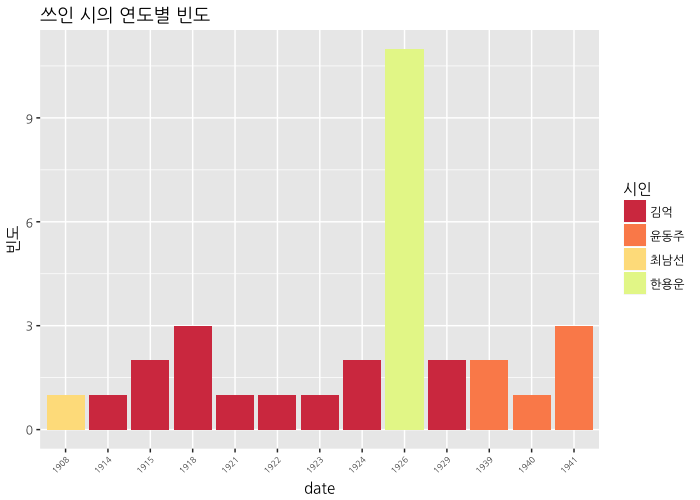
시가 많지 않아서 한해에 하나 정도밖에 없으니, 10년마다 묶도록 하겠습니다.
poet_table <- mutate(poet_table, decade=(as.numeric(as.character(date)) %/% 10) * 10)

head(poet_table, 10)
## poet date Freq decade
## 1 김억 1908 0 1900
## 2 윤동주 1908 0 1900
## 3 최남선 1908 1 1900
## 4 한용운 1908 0 1900
## 5 김억 1914 1 1910
## 6 윤동주 1914 0 1910
## 7 최남선 1914 0 1910
## 8 한용운 1914 0 1910
## 9 김억 1915 2 1910
## 10 윤동주 1915 0 1910
ggplot(data=poet_table, aes(x=decade, y=Freq, fill=factor(poet, levels=c("김억", "윤동주", "최남선", "한용운")))) +
  geom_bar(stat='identity', position='stack') +
  scale_fill_manual(values=RColorBrewer::brewer.pal(6, "Spectral")) +
  labs(x="연도", y="빈도",
       title="쓰인 시의 10년당 빈도") +
  guides(fill=guide_legend(title="시인")) +
  theme(axis.text.x=element_text(angle=45, size=6, hjust=1),
        text=element_text(family="NanumGothic"))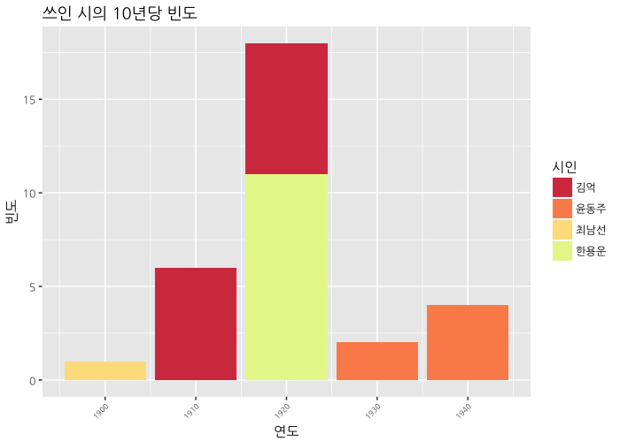
1920년대에 시가 편중되어 있어서 너무 아쉬웠습니다. 다음번엔 좀 더 많은 자료를 모아보겠습니다.
다음은 Bing 감정 점수입니다. 마찬가지로 10년 단위로 보겠습니다.
complete_data_frame_bing <- data_frame(date=as.numeric(unlist(poem_df$date)), score=scores) %>%
  mutate(decade=((date %/% 10) * 10)) %>%
  group_by(decade) %>%
  summarize(score=mean(score))

complete_data_frame_bing
## # A tibble: 5 × 2
## decade score
## <dbl> <dbl>
## 1 1900 -0.5128205
## 2 1910 0.1064437
## 3 1920 -0.2841417
## 4 1930 -0.7802964
## 5 1940 -0.2572544
ggplot(data=complete_data_frame_bing) +
  geom_bar(aes(x=decade, y=score, fill=score),
           stat="identity", position="identity") +
  ylim(-1, 1) +
  labs(y="평균 분율 점수", x="년도",
       title="Bing 감정 점수 분율의 막대그래프") +
  guides(fill=guide_legend(title="Bing 점수")) +
  theme(text=element_text(family="NanumGothic"))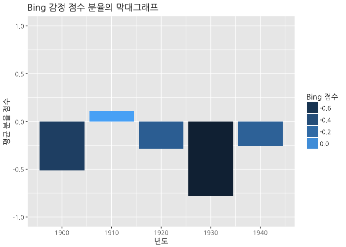
1900년대는 최남선 시인의 시 하나뿐이라서 좀 말하긴 어렵지만, 1930년대가 가장 어둡고 그 다음이 1900년대가 낮습니다. 오히려 1910년대는 좀 높게 나타나네요. 1930년대, 독립의 희망이 사라지던 시기에 가장 점수가 낮은 것은 그럴듯해 보입니다.
ggplot(data=complete_data_frame_bing) +
  geom_line(aes(x=decade, y=score), color="blue") +
  geom_point(aes(x=decade, y=score), size=1.3, color="blue") +
  ylim(-1, 1) +
  labs(y="평균 분율 점수", x="년도",
       title="Bing 감정 점수 분율의 선형그래프") +
  guides(fill=guide_legend(title="Bing 점수")) +
  theme(text=element_text(family="NanumGothic"))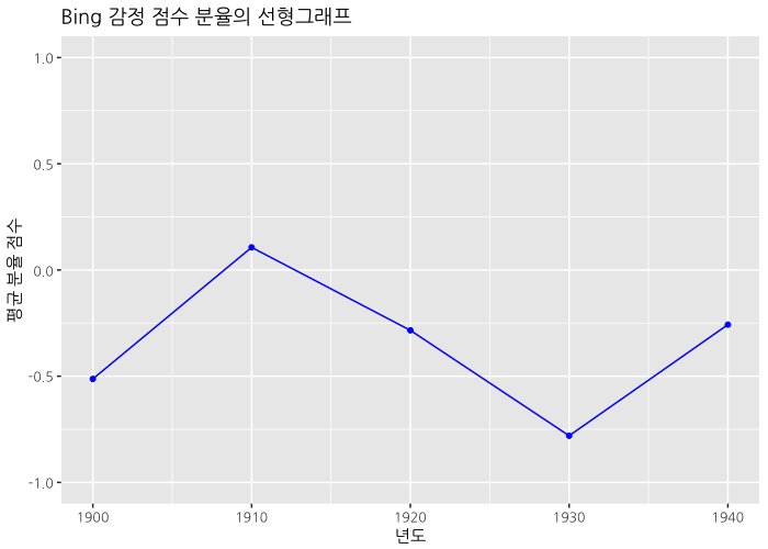
선형 그래프로 표현한 결과입니다.
bing_score_by_poet <- data_frame(poet=unlist(poem_df$poet), score=scores) %>%
  group_by(poet) %>%
  summarize(score=mean(score))

ggplot(data=bing_score_by_poet) +
  geom_bar(aes(x=reorder(poet, -score), y=score, fill=poet), stat="identity") +
  scale_fill_manual(values=RColorBrewer::brewer.pal(4, "Set1")) +
  labs(title="가장 부정적인 시를 발표한 시인은?",
       x="점수", y="시인") +
  guides(fill=guide_legend(title="시인")) +
  theme(text=element_text(family="NanumGothic"))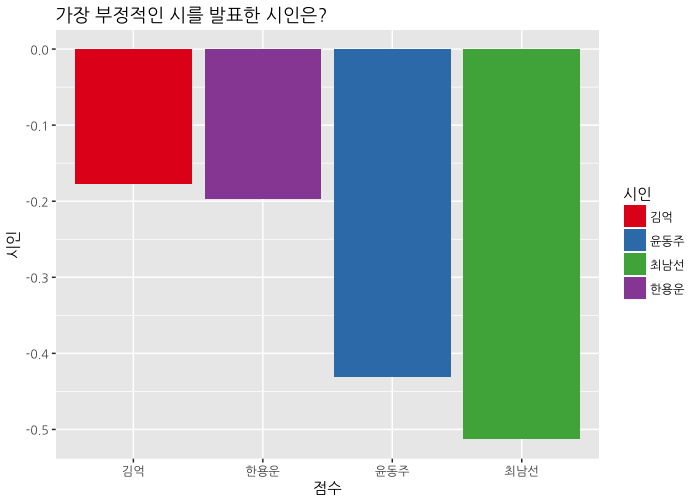
시인 별로 보면, 최남선 시인이 가장 부정적인 시어를 사용하고 있는 것을 볼 수 있습니다. “해에게서 소년에게”를 부정적인 시라고 보기는 어렵지만, 바다가 세상의 부정적인 것들에게 도전하고 있으며, 긍정의 표상인 바다와 파도는 의태어(“철썩”, “쏴아”)로만 제시되고 있으니 수긍할만 한 것 같습니다. 그래서 1900년대의 감정 점수가 낮군요.
다음은 NRC 감정 분석 결과입니다.
nrc_perdate <- nrc_analysis_df %>%
  mutate(decade=((as.numeric(date) %/% 10) * 10)) %>%
  group_by(decade, sentiment) %>%
  summarise(decadeSum=sum(value)) %>%
  mutate(decadeFreqPerc=decadeSum/sum(decadeSum))

head(nrc_perdate, 10)
## Source: local data frame [10 x 4]
## Groups: decade [2]
##
## decade sentiment decadeSum decadeFreqPerc
## <dbl> <chr> <int> <dbl>
## 1 1900 anger 3 0.13636364
## 2 1900 anticipation 3 0.13636364
## 3 1900 disgust 3 0.13636364
## 4 1900 fear 3 0.13636364
## 5 1900 joy 1 0.04545455
## 6 1900 sadness 3 0.13636364
## 7 1900 surprise 1 0.04545455
## 8 1900 trust 5 0.22727273
## 9 1910 anger 43 0.12500000
## 10 1910 anticipation 30 0.08720930
ggplot(data=nrc_perdate, aes(x=sentiment, y=decadeFreqPerc,
                             fill=sentiment)) +
  geom_bar(stat="identity") +
  scale_fill_brewer(palette="Spectral") +
  guides(fill=FALSE) +
  facet_wrap(~ decade, ncol=2) +
  theme(axis.text.x=element_text(angle=45, hjust=1, size=8),
        axis.title.y=element_text(margin=margin(0, 10, 0, 0)),
        plot.title=element_text(size=14)) +
  labs(x="감정", y="빈도 분율",
       title="연도별 감정 분율 막대 그래프") +
  theme(text=element_text(family="NanumGothic"))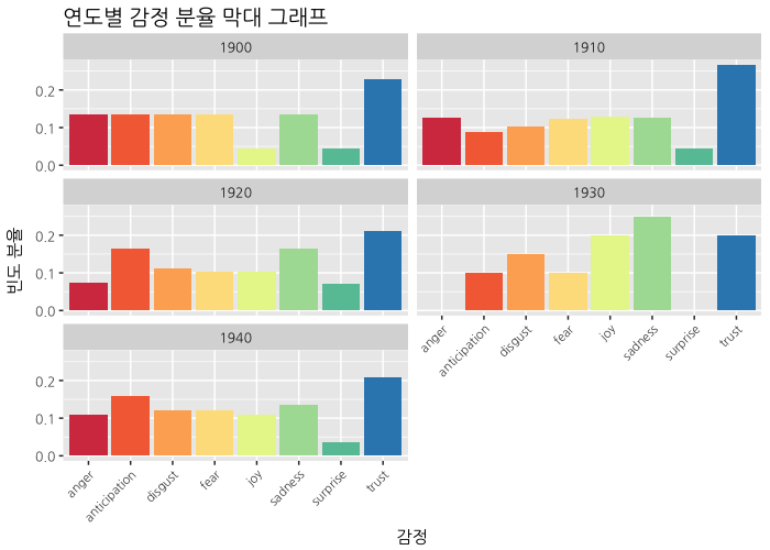
10년 단위로 본 NRC 감정 분석 그래프입니다. 1900년에서 1930년으로 가면서 분노는 점점 사라지고, 슬픔이 증가하는 것을 볼 수 있습니다. 1930년대에는 즐거움도 같이 증가하고 있다는 게 특징적입니다. 슬픔이 지나간 뒤의 기쁨에 관한 소망이 같이 표현되고 있기 때문일까요? 1920년대와 1940년대의 양상은 비슷하지만, 분노가 좀 더 높아졌네요. 전체적으로는 1930년대를 제외하면 신뢰가 가장 높게 나타납니다.
nrc_perpoet <- nrc_analysis_df %>%
  group_by(poet, sentiment) %>%
  summarise(poetSum=sum(value)) %>%
  mutate(dateFreqPerc=poetSum/sum(poetSum))

ggplot(data=nrc_perpoet, aes(x=sentiment, y=dateFreqPerc,
                             fill=sentiment)) +
  geom_bar(stat="identity") +
  scale_fill_brewer(palette="Spectral") +
  guides(fill=FALSE) +
  facet_wrap(~ poet, ncol=2) +
  theme(axis.text.x=element_text(angle=45, hjust=1, size=8),
        axis.title.y=element_text(margin=margin(0, 10, 0, 0)),
        plot.title=element_text(size=14)) +
  labs(y="빈도 분율", x="감정",
       title="시인별 감정 분율 막대 그래프") +
  theme(text=element_text(family="NanumGothic"))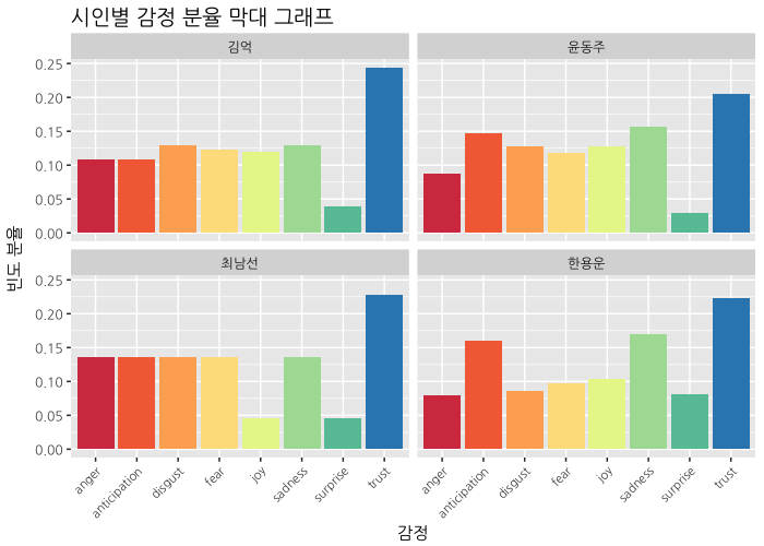
시인별 감정 분석입니다. 김억 시인은 전반적으로 비슷한데 신뢰가 가장 높고, 다음 혐오와 슬픔이 나타난다는 것이 특징입니다. 윤동주 시인은 기대와 슬픔이 좀 더 높으 편이고, 최남선 시인은 (역시) 즐거움은 별로 없고 나머지는 비슷합니다. 한용운 시인은 기대와 슬픔이 두드러지네요. 전체적으로 놀람이 잘 나타나지 않는데 한용운 시인에서 제일 높게 나타난 것을 볼 수 있습니다.
정리하며
분석에서 아쉬운 점이 많습니다.
- 감정 사전을 손봐야 합니다. 그대로 사용하기에는 아쉬운 점이 많이 있네요.
- 형태소 분석을 하지 않고 그냥 단어 별로 잘라서 분석하는 것도 가능합니다. 그러면 상당히 다른 형태의 결과가 나오게 됩니다만, 예컨대 윤동주 시인의 감정 점수가 긍정으로 나오기 때문에 받아들이기는 어려웠습니다. 형태소 분석을 하는 것이 더 낫지만(이것은 한국어가 영어처럼 띄어쓰기만으로 단어가 구분되지 않기 때문에 필요한 과정입니다) 단순히 명사만을 사용하는 것을 넘어 다른 형태소 또한 분석에 포함시키는 방법을 고민해야 할 것 같습니다.
- 자료가 너무 적어서, 다음번에는 좀 더 많은 시를 scraping하는 방법을 고민해야 할 것 같습니다. metadata를 같이 얻을 수 있는 사이트가 좋은데, 위키문헌에는 시만 올라와 있기 때문에 두 사이트를 같이 긁어와 결합하는 방법 등을 사용하는 부분을 생각해봐야 겠습니다.
좀 더 나은 결과물로 또 찾아뵙겠습니다.
Comments